With this coverage type, it is not the intention to test the system behaviour in separate situations, but to simulate the use of the system in a statistically responsible way. In order to test whether the system is proof against the realistic operation of it, that realistic operation needs to be specified one way or another. Such specifications are often called “profiles”. The 2 best-known are:

• Operational profiles - These describe which transactions are carried out by a user and with what frequency. The testing of operational profiles has the aim of examining whether: “The system continues to work correctly when transactions have been carried out often and over a long time”
• Load profiles - These describe the loading under which the system operates in terms of how many users are operating the system at once. The testing of load profiles has the aim of examining whether: “The system works correctly when many transactions are carried out by many users at once”

Both profiles are further explained below.

OPERATIONAL PROFILES

An operational profile describes in quantitative terms how the system is used by a particular type of user. This concept was introduced by John Musa; you are referred to his work [Musa, 1998] for a more comprehensive discussion of operational profiles. Below is a brief explanation.

An operational profile describes the realistic usage by answering the question: “When the system is in this condition, how great is the chance that this action will be carried out by the user?” In the literature, instead of condition and action, reference is usually made to history class and event. An operational profile provides a statistical average of how ‘the user’ handles the system. If various types of users are distinguishable who display significantly varied static average behaviour, it is advisable to create a separate operational profile per user type.

For example, for a system on “Internet banking” the following types of users could be distinguished:

• School pupils
• Adult consumers
• Business users

For the creation of an operational profile, the following steps are gone through:

1. Determine the list of possible events - This covers, in principle, all the actions and events with which the system functionality is activated. These are usually the functions that are carried out by users or connected systems. If various functions have been defined that have a lot to do with each other and which also have the same likelihood of being executed, it is advisable to group these functions. This keeps the operational profile clear.
2. Determine the history classes of the system - A history class describes the condition in which the system finds itself. It says something about what has happened (the history) with the system. The occurrence of an event (execution of a function) usually results in the system arriving in a different history class.
   
   For example, for a DVD recorder the history classes defined are “Standby”, “Record”, “Play”, “Fast Forward”, and “Fast Rewind”. If, in the history class of “Play” the user presses the “Forward” button (an event), the system moves into the history class of “Fast Forward”. However, if the user presses this button in the history class of “Record”, this has no effect and the system remains in the same history class.

   In general, it is advisable to nominate a new history class if the probability distribution in respect of the occurrence of the subsequent event changes significantly. It is usual for the first history class to select the initial condition of the system.

3. Determine for each history class the probability distribution of the events - In other words: how great are the chances that this event will be executed if the system is in this history class. In every history class, the sum of all the probabilities should come out as 1 (or 100%).

The result of these steps can be reproduced in the form of a matrix, as illustrated in figure 1. In this, for example, the term P2,1 means “the chances that event 1 will be executed by the user in history class 2”.

Figure 1: General content of an operational profile.

There are various ways of obtaining the information required for an operational profile, for example:

• Copying an existing operational profile of a system with similar functionality (e.g. the preceding system)
• Maintaining data (logging) on how often each function is used
• Interviewing users.

It is important here to realise that this does not concern ‘100% accurate measurements’, but estimates that provide a realistic impression of the average use of the system.

Testing operational profiles

A test case consists in this instance of a chain of events that are carried out by the user. The length of a test case is up to the tester, but typically is in the order of some tens of events in sequence. The test case starts in the initial condition (history class 1). Subsequently, the system will move into other history classes, depending on the events that are carried out.

For the creation of each test case, the following steps are performed:

1. Start in history class 1
2. Select the following event to be carried out - This is derived directly from the operational profile. With the aid of a random generator, a figure between 0 and 100% is generated and the corresponding event from the operational profile is determined. This results in events occurring in a statistically responsible manner in the test set with large numbers of test cases (in accordance with the probability distribution in the operational profile).
3. Determine into which subsequent history class the system consequently arrives - This is determined by how the system functions. It should therefore be derived from the functional specifications of the system.
4. Repeat steps 2 and 3 until the required length of the test case has been reached.

In order to test the realistic usage in a statistically responsible way according to the operational profile, a large number of test cases is required, each carrying out a large number of actions (events). This is more or less impossible to do manually. It is advisable to generate the required test cases automatically. This is not further discussed here, but more information on it can be found in the book “Testing Embedded Software” [Broekman, 2003], among other sources.

LOAD PROFILES

Load profiles show the degree to which the system resources (CPU, memory, network capacity) are loaded in reality. The loading is usually shown in terms of the number of users or number of times that a transaction is carried out in a particular period. Usually, the loading of a system is not continuously even, but varies over a period of time: there are peaks and valleys within a 24-hour stretch. Often, weekends will show a different loading from weekdays. And during holiday periods and public holidays, the loading of a system may look different again. In figure 1, an example is shown of a load profile over the course of 24 hours.

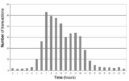
Figure 2: Example of a load profile, showing the number of transactions per hour over a full 24-hour period.

• Measuring the loading of the system using specific tools (monitors) - The responsibility for this usually resides with a department for “Technical System Administration”
• Interviewing users - In fact, this amount to the following questions: “Which transactions do you carry out? How often, and when?”

Testing load profiles

The testing of load profiles comes under the category of “performance testing” and is a testing specialism in itself. While it is possible to do manually, tools are usually employed that generate a particular loading of the system. Using the tools, a realistic loading is simulated, such as:

• Creation of virtual users - A virtual user is a small program that simulates a user. On one PC, many such programs can run at once. This avoids the need for the physical presence of a separate PC for each user. This is mainly applied for subjecting the entire system, including the network, to a particular loading
• Offering transactions via the database-management interface - This creates a certain loading of the back-end of the system without overloading the front-end or the network. It facilitates direct measurement of whether the database server has the appropriate dimensions.

There are various types of performance tests that each have a different goal. The most common are:

• Testing with normal or average usage - The aim here is to examine whether the available system resources are adequate for the ‘usual’ circumstances. The idea here is, that it can be commercially advantageous to deploy extra resources for the rare occasions that ‘exceptionally heavy loading’ takes place.
• Testing with peak loading - The aim here is to examine whether there are sufficient system resources for even the most demanding circumstances that may arise in practice.
• Measuring the breaking point - This is also known as “stress testing”. The aim here is to examine what the maximum load is under which the system will still perform acceptably. With a particular system configuration, the loading is stepped up, while the response time is measured. This can be shown in a graph. At the point when the graph shows a sharp incline, the response time increases disproportionately fast (the response ‘collapses’) and the breaking point has been reached.

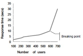
Figure 3: Example of the measurement of the breaking point: the maximum load at which the system still performs at an acceptable level.